2D Example

In this example, we use the pulsarfitpy library to analyze the following differential equation relating to pulsar spindown:
2D Differential Equation

The sample Python code shows how we analyzed this equation with multiple graphs using pulsarfitpy and other Python modules together.

"""
Example Usage of 2D Physics-Informed Neural Networks for Pulsar Modeling

This script demonstrates how to use the PulsarPINN2D framework to solve
a 2D partial differential equation modeling pulsar magnetospheric dynamics.
We query real pulsar data from the ATNF Catalog using psrqpy and use it to
train a physics-informed neural network to learn relationships between
pulsar physical parameters.

The model relates three key pulsar parameters:
- Period (P): Pulsar rotation period in seconds
- Period Derivative (dP/dt): Rate of period change
- Surface Magnetic Field (B): Calculated from P and dP/dt

A simplified 2D PDE models how the magnetic field evolves as a function
of both period and spin-down characteristics.

Author: pulsarfitpy Development Team
License: MIT
"""

First, we setup the program by importing the necessary libraries for the project. In this case, it will be numpy, sympy, psrqpy, matplotlib, warnings, and pulsarfitpy.

import numpy as np
import sympy as sp
import matplotlib.pyplot as plt
import warnings

# Suppress warnings for cleaner output
warnings.filterwarnings('ignore')

# Import 2D PINN framework
from pulsarfitpy import PulsarPINN2D, Backend

Now, we begin the setup for the equation. We import the proper pulsar data using psrqpy, extract and process it, and organize the data together.

# ============================================================================
# EXECUTION BEGINS HERE
# ============================================================================

print("\n" + "="*80)
print("2D Physics-Informed Neural Network for Pulsar Parameter Modeling")
print("="*80)

# Step 1: Query real pulsar data from ATNF
print("\nStep 1: Loading pulsar data")
print("-" * 80)

print("\n" + "="*80)
print("Querying ATNF Pulsar Catalog")
print("="*80 + "\n")

import psrqpy

# Query the ATNF catalog
query = psrqpy.QueryATNF(params=['NAME', 'P0', 'P1', 'BSURF'])

# Access the pandas DataFrame directly (not a callable method)
pulsars = query.pandas

# Select pulsars with valid data
valid_mask = (
    pulsars['P0'].notna() & 
    pulsars['P1'].notna() & 
    pulsars['BSURF'].notna() &
    (pulsars['P0'] > 0) &
    (pulsars['P1'] > 0) &
    (pulsars['BSURF'] > 0)
)

valid_pulsars = pulsars[valid_mask].head(40)

# Extract data
names = valid_pulsars['NAME'].values.tolist()
period = valid_pulsars['P0'].values
period_dot = valid_pulsars['P1'].values
magnetic_field = valid_pulsars['BSURF'].values

# Convert to logarithmic scale for better numerical stability
log_period = np.log10(period)
log_period_dot = np.log10(period_dot)
log_magnetic_field = np.log10(magnetic_field)

print(f"Successfully retrieved {len(names)} pulsars from ATNF")
print(f"\nPulsar data summary:")
print(f"  Period range: {period.min():.4e} to {period.max():.4e} seconds")
print(f"  Period derivative range: {period_dot.min():.4e} to {period_dot.max():.4e} s/s")
print(f"  Magnetic field range: {magnetic_field.min():.4e} to {magnetic_field.max():.4e} Gauss")

pulsar_data = {
    'names': names,
    'period': period,
    'period_dot': period_dot,
    'magnetic_field': magnetic_field,
    'log_period': log_period,
    'log_period_dot': log_period_dot,
    'log_magnetic_field': log_magnetic_field
}

Next we start with the model. We define the equation using sympy symbols and recreate our physics constraint.

# Step 2: Define the 2D PDE model
print("\nStep 2: Defining pulsar magnetospheric PDE")
print("-" * 80)

# Define symbolic variables for input space (what PINN receives)
log_P = sp.Symbol('log_P', real=True)
log_Pdot = sp.Symbol('log_Pdot', real=True)
log_B = sp.Symbol('log_B', real=True)

# Define learnable constants
alpha = sp.Symbol('alpha', real=True)
beta = sp.Symbol('beta', real=True)
gamma = sp.Symbol('gamma', real=True)

# Physics constraint: log(B) = gamma + alpha*log(P) + beta*log(dP/dt)
# Rearranged to constraint form: log(B) - gamma - alpha*log(P) - beta*log(dP/dt) = 0
# This ensures the network learns the relationship between parameters
pde_expr = log_B - gamma - alpha * log_P - beta * log_Pdot

print(f"PDE formulation:\n  {pde_expr} = 0\n")
print("This PDE models magnetic field evolution in the period-spin-down space")
print("The PINN will learn constants alpha and beta that characterize")
print("how the magnetic field depends on pulsar rotation properties.\n")

Now, we prepare the data to use in the model using numpy.

# Step 3: Prepare training data
print("Step 3: Preparing training data from observations")
print("-" * 80)

# Extract log-scale data
log_P_data = pulsar_data['log_period']
log_Pdot_data = pulsar_data['log_period_dot']
log_B_data = pulsar_data['log_magnetic_field']

# Number of pulsars
n_pulsars = len(log_P_data)
n_test = max(1, int(n_pulsars * 0.2))
n_train = n_pulsars - n_test

# Randomly select training and testing data
indices = np.arange(n_pulsars)
np.random.shuffle(indices)

train_indices = indices[:n_train]
test_indices = indices[n_train:]

# Use training pulsars as boundary conditions (observed values)
boundary_points = np.column_stack([
    log_P_data[train_indices],
    log_Pdot_data[train_indices]
])
boundary_values = log_B_data[train_indices]

# Create interior collocation points via interpolation
# Generate a denser grid of points within the observed parameter space
log_P_min, log_P_max = log_P_data.min(), log_P_data.max()
log_Pdot_min, log_Pdot_max = log_Pdot_data.min(), log_Pdot_data.max()

# Create a regular grid and add some random perturbation
n_grid = int(np.sqrt(n_train * 2))
P_grid = np.linspace(log_P_min, log_P_max, n_grid)
Pdot_grid = np.linspace(log_Pdot_min, log_Pdot_max, n_grid)
P_mesh, Pdot_mesh = np.meshgrid(P_grid, Pdot_grid)

collocation_points = np.column_stack([
    P_mesh.flatten(),
    Pdot_mesh.flatten()
])

# Add some random noise to collocation points for better coverage
random_points = np.random.rand(n_train, 2)
random_points[:, 0] = random_points[:, 0] * (log_P_max - log_P_min) + log_P_min
random_points[:, 1] = random_points[:, 1] * (log_Pdot_max - log_Pdot_min) + log_Pdot_min

collocation_points = np.vstack([collocation_points, random_points])

print(f"\nTraining data prepared:")
print(f"  Collocation points: {len(collocation_points)}")
print(f"  Boundary points: {len(boundary_points)}")
print(f"  Test pulsars (excluded from training): {len(test_indices)}")

Now, we initialize the 2D PINN using the PulsarPINN2D class.

# Step 4: Initialize the 2D PINN
print("\nStep 4: Initializing 2D Physics-Informed Neural Network")
print("-" * 80)

pinn_2d = PulsarPINN2D(
    pde_expr=pde_expr,
    input_dim=2,
    hidden_layers=[64, 64, 64],
    output_dim=1,
    backend=Backend.PYTORCH,
    device='cpu'
)

We load the training data into the 2D PINN using the set_training_data method.

# Step 5: Set training data
print("\nStep 5: Loading training data into PINN")
print("-" * 80)
pinn_2d.set_training_data(
    collocation_points=collocation_points,
    boundary_points=boundary_points,
    boundary_values=boundary_values
)
print("Training data loaded successfully\n")

Now, we configure the visualization settings for the graphs using the set_visualization_config method.

# Step 6: Configure visualization
print("Step 6: Configuring visualization settings")
print("-" * 80)
pinn_2d.set_visualization_config(
    colormap='plasma',
    dpi=150,
    figsize=(12, 9)
)
print("Visualization configured for publication quality\n")

Now, we train the PINN using the train method.

# Step 7: Train the PINN
print("Step 7: Training the Physics-Informed Neural Network")
print("-" * 80)
print("Training will minimize both:")
print("  - Physics loss: How well the PDE is satisfied")
print("  - Data loss: How well observations are matched")
print("Starting training...\n")

metrics_history = pinn_2d.train(
    epochs=10000,
    learning_rate=1e-3,
    callback_interval=200
)

print("\nTraining completed!\n")

Now, we analyze the data and evaluate it using the get_metrics_summary method.

# Step 8: Evaluate results
print("Step 8: Analyzing trained model")
print("-" * 80)

metrics_summary = pinn_2d.get_metrics_summary()

# Extract final metrics from training history
if metrics_history:
    final_metrics = metrics_history[-1]
    print(f"\nFinal Training Metrics:")
    print(f"  Final total loss: {final_metrics.total_loss:.6e}")
    print(f"  Final physics loss: {final_metrics.pde_loss:.6e}")
    print(f"  Final data loss: {final_metrics.boundary_loss:.6e}\n")
else:
    print("No training metrics available\n")

Now, we start generating the visualizations.

# Step 9: Generate visualizations
print("Step 9: Generating analysis visualizations")
print("-" * 80)

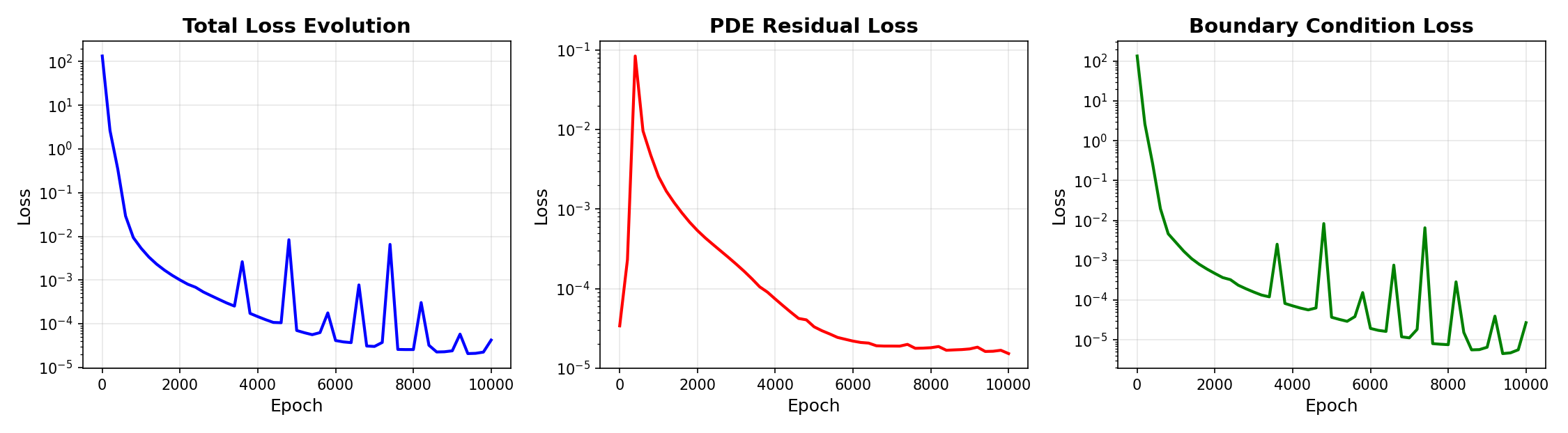
We plot the loss history using the plot_loss_history graph.

# Plot training loss evolution
print("  Generating loss history plot...")
pinn_2d.plot_loss_history(
    log_scale=True,
    separate_losses=True,
    savefig=None
)
plt.show()

2D Loss History Graph

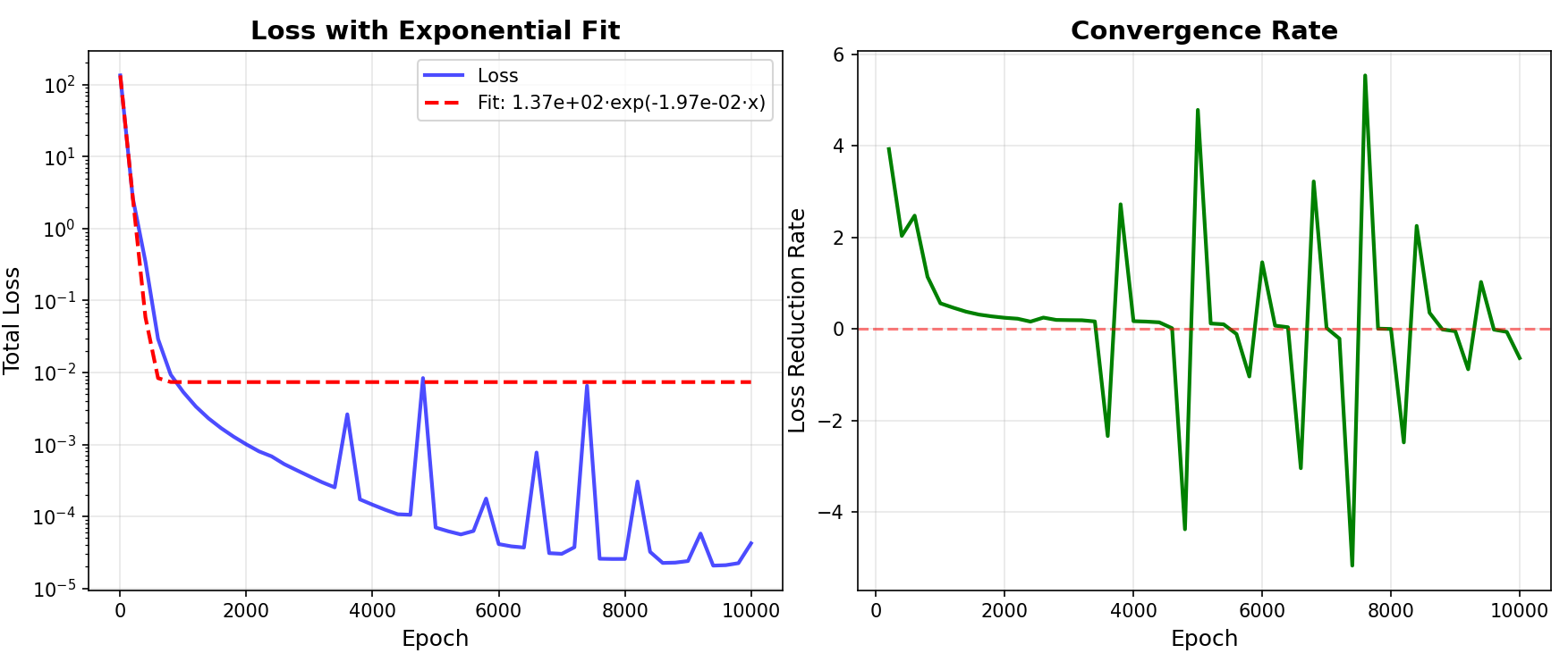
Using the plot_convergence_rate method, we plot convergence analysis.

# Plot loss convergence analysis
print("  Generating convergence analysis...")
pinn_2d.plot_convergence_rate(
    savefig=None
)
plt.show()

Convergence Rate Graph

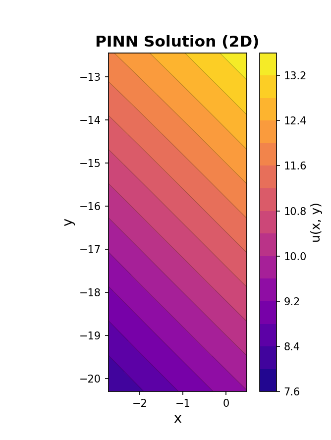
Now we plot the solution contour plot using plot_solution_2d.

# Plot the learned 2D solution surface
print("  Generating 2D solution contour plot...")
pinn_2d.plot_solution_2d(
    resolution=100,
    x_range=(pulsar_data['log_period'].min(), pulsar_data['log_period'].max()),
    y_range=(pulsar_data['log_period_dot'].min(), pulsar_data['log_period_dot'].max()),
    colormap='plasma',
    savefig=None
)
plt.show()

2D Solution Plot

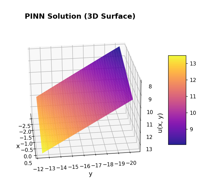
Now, we use plot_solution_3d to plot a 3D surface visualization.

# Plot 3D surface representation
print("  Generating 3D surface visualization...")
pinn_2d.plot_solution_3d(
    resolution=80,
    x_range=(pulsar_data['log_period'].min(), pulsar_data['log_period'].max()),
    y_range=(pulsar_data['log_period_dot'].min(), pulsar_data['log_period_dot'].max()),
    elevation=25,
    azimuth=45,
    savefig=None
)
plt.show()

3D Surface Visualization

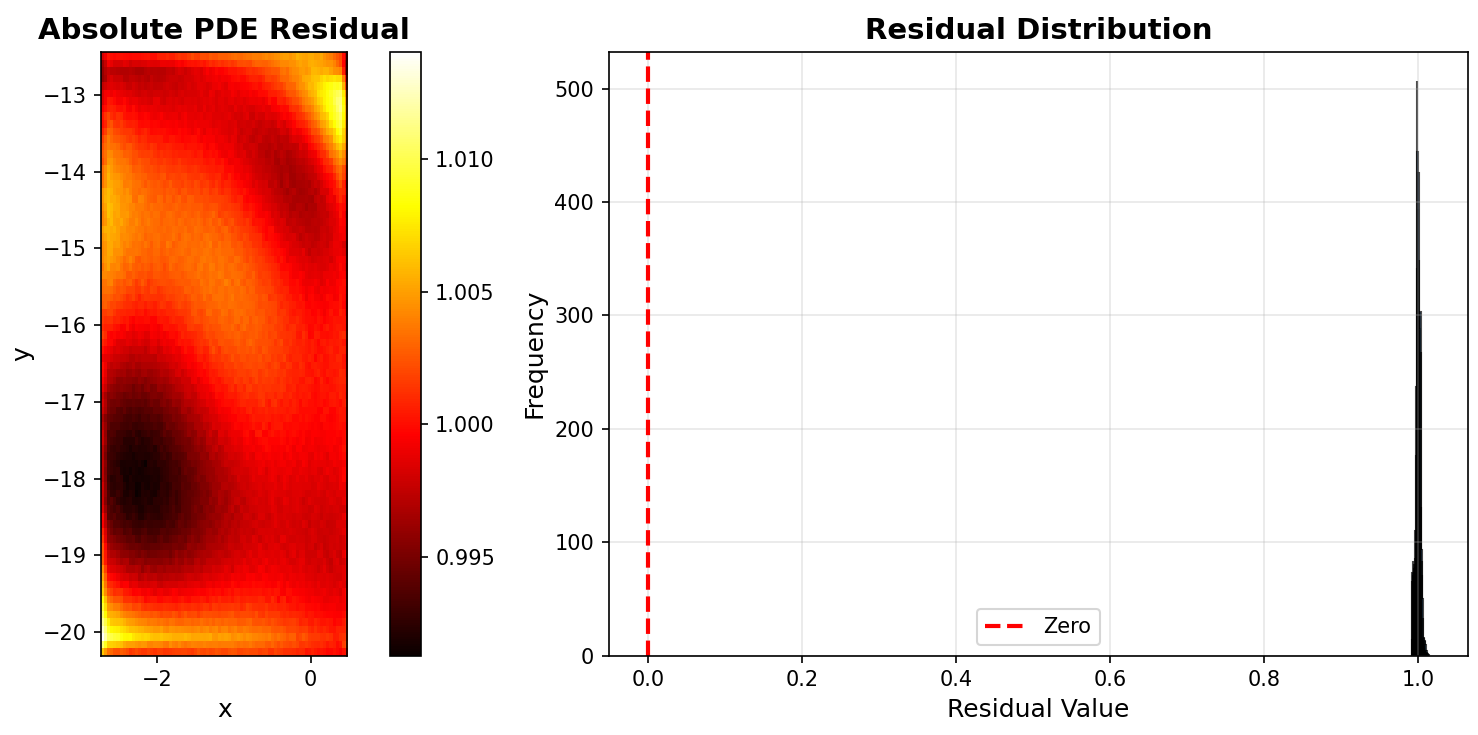
Now, we plot PDE residual distribution using plot_residual_distribution.

# Plot residual distribution
print("  Generating PDE residual distribution...")
pinn_2d.plot_residual_distribution(
    resolution=80,
    x_range=(pulsar_data['log_period'].min(), pulsar_data['log_period'].max()),
    y_range=(pulsar_data['log_period_dot'].min(), pulsar_data['log_period_dot'].max()),
    savefig=None
)
plt.show()

print("\nAll visualizations displayed successfully!")

Residual Distribution Graph

Now that all our visualizations are complete, we make predictions with the model.

# Step 10: Demonstrate prediction capability
print("Step 10: Making predictions with trained model")
print("-" * 80)

test_log_P = np.array([2.0, 0.5, -1.0])
test_log_Pdot = np.array([-15.0, -18.0, -20.0])

predictions = pinn_2d.predict(test_log_P, test_log_Pdot)

print("\nSample predictions for new parameter combinations:")
for i in range(len(test_log_P)):
    P = 10.0 ** test_log_P[i]
    Pdot = 10.0 ** test_log_Pdot[i]
    B = 10.0 ** predictions[i]
    print(f"  Period {P:.4e} s, dP/dt {Pdot:.4e} s/s -> B = {B:.4e} Gauss")

Finally, we save the model using the save_model method.

# Step 11: Save the trained model
print("\nStep 11: Persisting trained model")
print("-" * 80)
pinn_2d.save_model('pulsar_pinn_2d_model.pt')
print("Model saved to pulsar_pinn_2d_model.pt\n")

print("="*80)
print("2D PINN Training Complete!")
print("="*80)

Next Steps

Explore the Technical Information
Check out the Jupyter notebooks in src/pulsarfitpy/docs/

← Back to Examples Home