1D Example

In this example, we use the pulsarfitpy library to analyze the following differential equation relating to pulsar spindown:

The sample Python code shows how we analyzed this equation with multiple graphs using pulsarfitpy and other Python modules together.

First, we begin by importing the necessary Python modules we will need for this project. In this case, it will be numpy, sympy, psrqpy, and pulsarfitpy.

"""
PINN Test Script for Pulsar Spindown Analysis
Author: Om Kasar & Saumil Sharma
Date: December 2025
"""

import numpy as np
import sympy as sp
from pulsarfitpy import PulsarPINN, VisualizePINN, ExportPINN
from psrqpy import QueryATNF

With all the Python libraries imported and ready, query the data from the ATNF database. In this code segment, we query for pulsars that have valid entries for period and period derivative and converted each into logarithmic scale.

# =============================================================================
# STEP 1: QUERY PULSAR SPINDOWN DATA FROM ATNF
# =============================================================================

# Query the ATNF pulsar catalog for period and period derivative
query = QueryATNF(params=['P0', 'P1', 'ASSOC'])
query_table = query.table

# Extract valid data: filter out pulsars with missing P0 or P1 values
filter = (query_table['P0'].mask) & (query_table['P1'].mask)
P = query_table['P0'][filter].data  # Period in seconds
Pdot = query_table['P1'][filter].data  # Period derivative (s/s)

# Convert to log scale
log_P = np.log10(P)
log_Pdot = np.log10(np.abs(Pdot))

# Remove any remaining NaN or inf values
valid_data = np.isfinite(log_P) & np.isfinite(log_Pdot)
log_P = log_P[valid_data]
log_Pdot = log_Pdot[valid_data]

print(f"Queried {len(log_P)} pulsars with valid P and Pdot measurements from ATNF catalog")

After querying the necessary parameters, we use sympy to define the symbols for each part of the differential equation and the equation itself.

# =============================================================================
# STEP 2: DEFINE SYMBOLIC DIFFERENTIAL EQUATION FOR SPINDOWN
# =============================================================================

logP = sp.Symbol('logP')
logPdot = sp.Symbol('logPdot')
n_braking = sp.Symbol('n_braking')
logK = sp.Symbol('logK')

differential_equation = sp.Eq(logPdot, (n_braking - 1) * logP + logK)

After establishing the equation, we now input all the information into the PulsarPINN class.

# =============================================================================
# STEP 3: INITIALIZE PINN WITH SPINDOWN MODEL
# =============================================================================

fixed_inputs = {
    logP: log_P,
    logPdot: log_Pdot
}

pinn = PulsarPINN(
    differential_eq=differential_equation,
    x_sym=logP,
    y_sym=logPdot,
    learn_constants={
        n_braking: 2.1,
        logK: -16.0
    },
    fixed_inputs=fixed_inputs,
    log_scale=True,
    input_layer=1,
    hidden_layers=[64, 32],
    output_layer=1,
    train_split=0.70,
    val_split=0.15,
    test_split=0.15,
    random_seed=42
)

Now we train the PINN using the train method of the PulsarPINN class.

# =============================================================================
# STEP 4: TRAIN THE PINN
# =============================================================================

pinn.train(
    epochs=6000,
    training_reports=600,
    physics_weight=1.0,
    data_weight=1.0
)

We analyze the model and calculate if it is a good fit using various metrics of the evaluate_test_set function. Setting verbose to True will enumerate the details.

# =============================================================================
# STEP 5: EVALUATE MODEL PERFORMANCE
# =============================================================================

print("\n\n")
print("*" * 80)
print("MODEL EVALUATION")
print("*" * 80)
print()

metrics = pinn.evaluate_test_set(verbose=True)

Now we print the learned constants the model derived from the data and differential equation using the store_learned_constants method.

# =============================================================================
# STEP 6: ANALYZE LEARNED PHYSICAL CONSTANTS
# =============================================================================

learned_constants = pinn.store_learned_constants()
learned_n = learned_constants['n_braking']
learned_logK = learned_constants['logK']

print("\n" + "=" * 80)
print("LEARNED PHYSICAL CONSTANTS")
print("=" * 80)
print(f"\nBraking Index: n = {learned_n:.6f}")
print(f"Spindown Constant: log(K) = {learned_logK:.6f}")

After storing the constants, we test the uncertainty using the bootstrap_uncertainty method of the PulsarPINN class.

# =============================================================================
# STEP 7: UNCERTAINTY QUANTIFICATION
# =============================================================================

print("\n\n")
print("*" * 80)
print("UNCERTAINTY QUANTIFICATION (BOOTSTRAP)")
print("*" * 80)
print()

uncertainties = pinn.bootstrap_uncertainty(
    n_bootstrap=50,
    sample_fraction=0.9,
    epochs=1500,
    confidence_level=0.95,
    verbose=True
)

After using bootstrap sampling to determine uncertainty, we run robustness tests using the run_all_robustness_tests method.

# =============================================================================
# STEP 8: ROBUSTNESS VALIDATION
# =============================================================================

print("\n\n")
print("*" * 80)
print("ROBUSTNESS VALIDATION (PERMUTATION, SHUFFLING, PHYSICS TESTS)")
print("*" * 80)
print()

robustness_results = pinn.run_all_robustness_tests(
    n_permutations=50,
    n_shuffles=50,
    verbose=True
)

Using the VisualizePINN method, we plot various graphs of our results including predictions vs data, loss curves, residuals analysis, residuals scatter, braking distribution index distribution, uncertainty quantification, and robustness validation.

# =============================================================================
# STEP 9: VISUALIZATION AND ANALYSIS
# =============================================================================

print("\n\n")
print("*" * 80)
print("VISUALIZATION AND ANALYSIS")
print("*" * 80)
print()

# Initialize visualizer
visualizer = VisualizePINN(pinn)

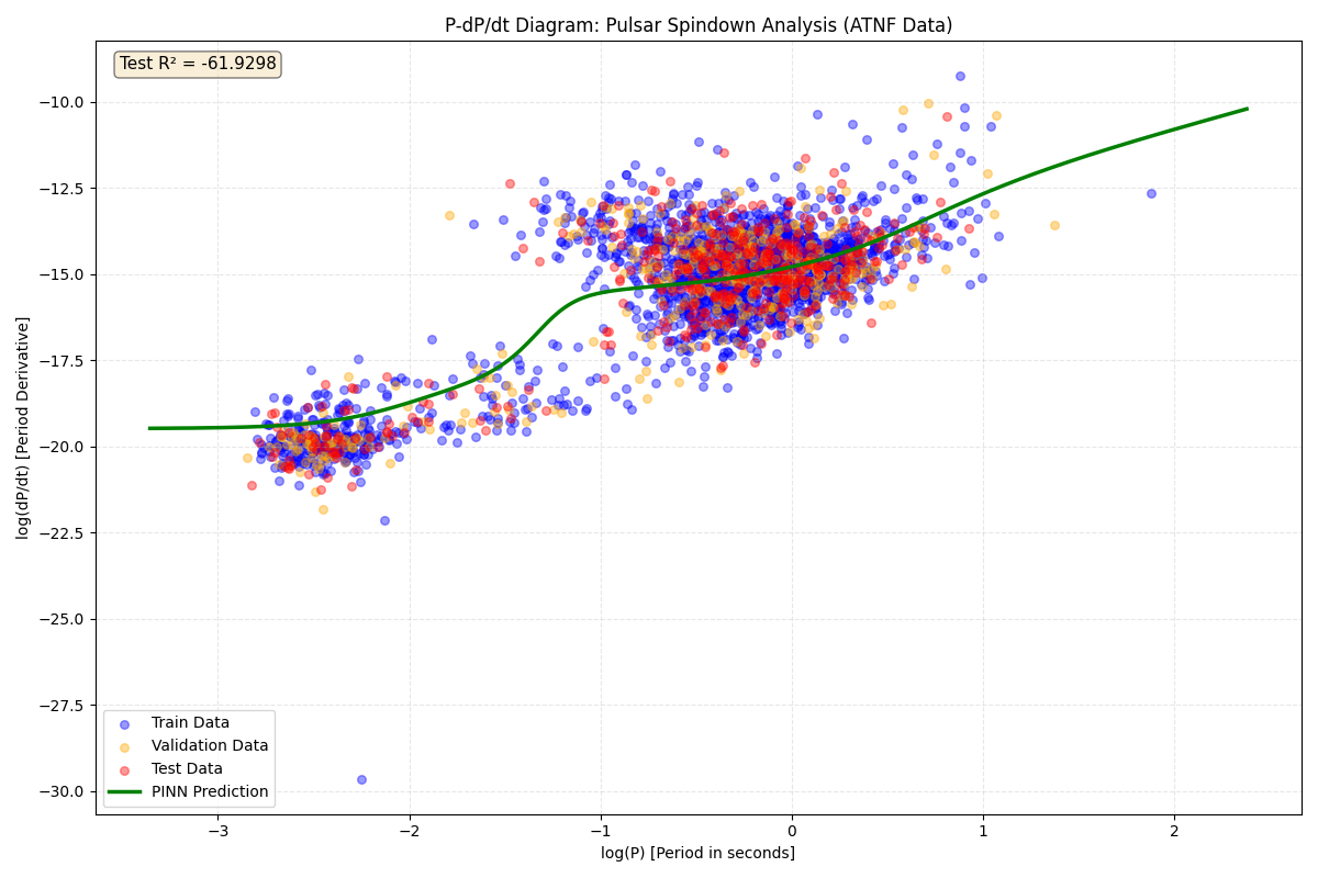
# Plot 1: Predictions vs Data
visualizer.plot_predictions_vs_data(
    x_axis='log(P) [Period in seconds]',
    y_axis='log(dP/dt) [Period Derivative]',
    title='P-dP/dt Diagram: Pulsar Spindown Analysis (ATNF Data)'
)

Predictions vs Data Graph

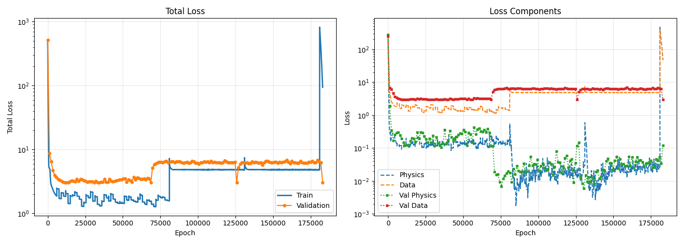
# Plot 2: Training and Validation Loss Curves
visualizer.plot_loss_curves(log_scale=True)

Loss Curves Graphs

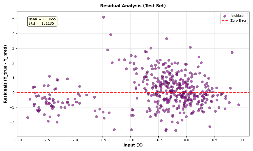
# Plot 3: Residuals Analysis
visualizer.plot_residuals_analysis()

Residuals Analysis

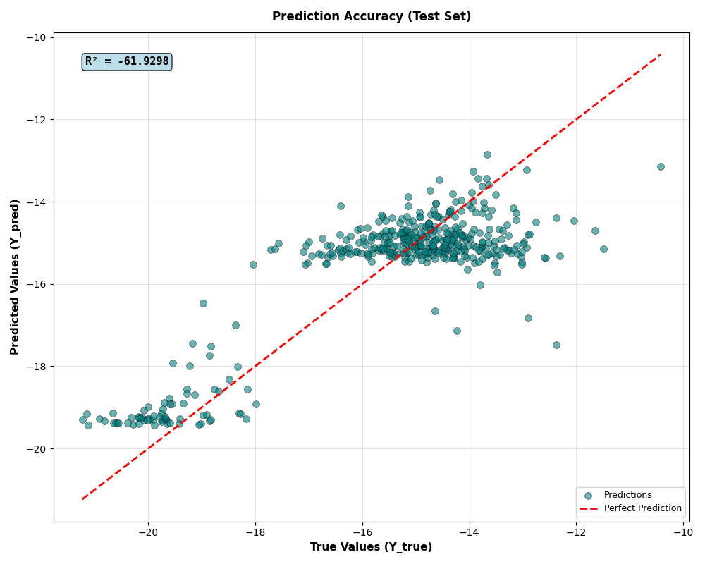
# Plot 4: Prediction Scatter Plot
visualizer.plot_prediction_scatter()

Prediction Scatter

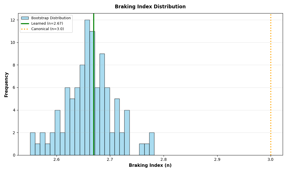
# Plot 5: Braking Index Distribution
visualizer.plot_braking_index_distribution(
    learned_constants=learned_constants,
    uncertainties=uncertainties
)

Braking Index Distribution

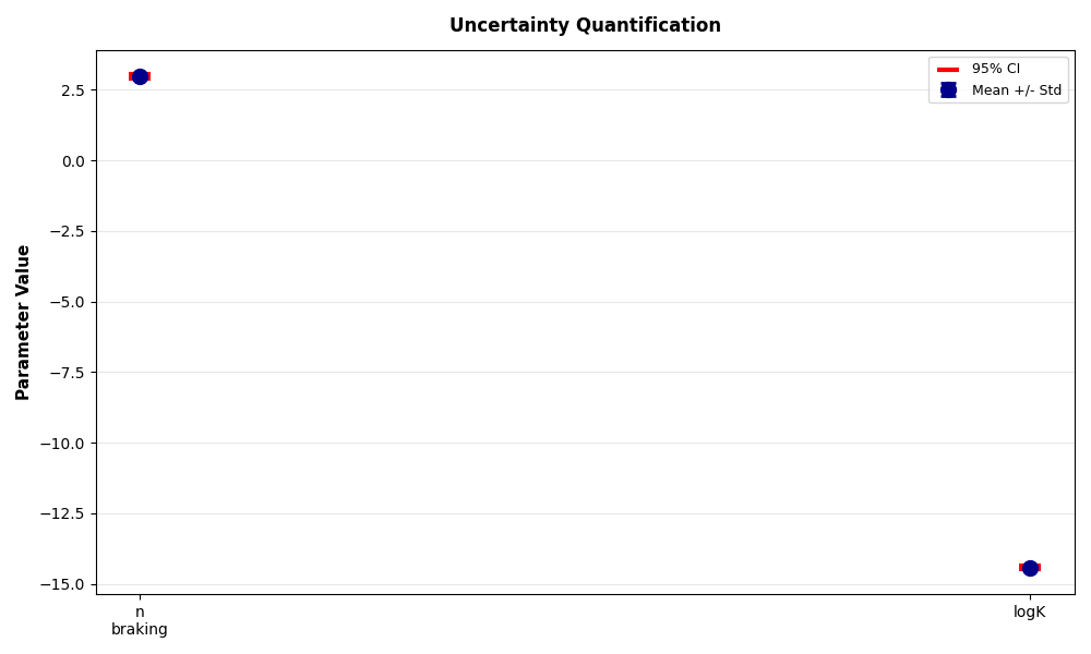
# Plot 6: Uncertainty Quantification
visualizer.plot_uncertainty_quantification(uncertainties=uncertainties)

Uncertainty Quantification

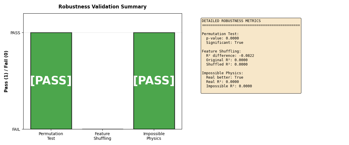
# Plot 7: Robustness Validation
visualizer.plot_robustness_validation(robustness_results=robustness_results)

Robustness Validation

Now we use the ExportPINN class’s methods to save the results to CSV files.

# =============================================================================
# STEP 10: EXPORT RESULTS TO CSV FILES
# =============================================================================

print("\n\n")
print("*" * 80)
print("EXPORTING RESULTS TO CSV")
print("*" * 80)
print()

# Initialize exporter
exporter = ExportPINN(pinn)

# Export predictions with raw data and test metrics
exporter.save_predictions_to_csv(
    filepath='data/outputs/pinn_predictions.csv',
    x_value_name='log_period',
    y_value_name='log_period_derivative',
    include_raw_data=True,
    include_test_metrics=True,
    additional_metadata={
        'model_type': 'Pulsar Spindown PINN',
        'data_source': 'ATNF Pulsar Catalog',
        'n_pulsars_used': len(log_P)
    }
)

# Export learned constants with uncertainty estimates from bootstrap
exporter.save_learned_constants_to_csv(
    filepath='data/outputs/learned_constants.csv',
    include_uncertainty=True,
    uncertainty_method='bootstrap',
    n_iterations=50,
    additional_info={
        'model': 'pulsar_spindown',
        'equation': str(differential_equation),
        'training_epochs': 6000
    }
)

# Export evaluation metrics
exporter.save_metrics_to_csv(
    filepath='data/outputs/evaluation_metrics.csv',
    additional_info={
        'test_set_size': len(pinn.x_test),
        'train_set_size': len(pinn.x_train),
        'val_set_size': len(pinn.x_val),
        'total_samples': len(log_P)
    }
)

# Export training loss history
exporter.save_loss_history_to_csv(
    filepath='data/outputs/loss_history.csv'
)

print("CSV export complete. Files saved to data/outputs/")
print("  - pinn_predictions.csv: Model predictions with raw data")
print("  - learned_constants.csv: Learned constants with uncertainty")
print("  - evaluation_metrics.csv: Test/train/val performance metrics")
print("  - loss_history.csv: Training loss history")

Finally, we print a summary report of the data.

# =============================================================================
# STEP 11: COMPREHENSIVE SUMMARY REPORT
# =============================================================================

print("\n\n")
print("*" * 80)
print("FINAL SUMMARY AND RESULTS")
print("*" * 80)
print()

print("\n" + "=" * 80)
print("FINAL SUMMARY")
print("=" * 80)
print(f"\nTest R2: {metrics['test_r2']:.6f}")
print(f"Test RMSE: {metrics['test_rmse']:.6e}")
print(f"Test MAE: {metrics['test_mae']:.6e}")
print(f"\nn = {learned_n:.4f} +/- {uncertainties['n_braking']['std']:.4f}")
print(f"95% CI: [{uncertainties['n_braking']['ci_lower']:.4f}, {uncertainties['n_braking']['ci_upper']:.4f}]")
print(f"log(K) = {learned_logK:.4f} +/- {uncertainties['logK']['std']:.4f}")
print("\n" + "=" * 80)

Figure 1 Data
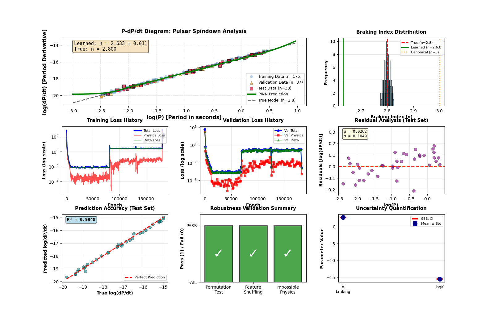
A collection of all the graphs created through the visualizer feature of pulsarfitpy.

Common Parameters

pulsarfitpy offers analysis of other pulsar properties outside of those outlined in the example. Some common parameters are listed in the table below.

Parameter	Description
`P0`	Pulsar period (s)
`P1`	Period derivative (s/s)
`DM`	Dispersion measure (pc/cm³)
`BSURF`	Surface magnetic field (G)
`EDOT`	Spin-down energy loss rate (erg/s)

For further analysis of pulsar properties, see the ATNF Pulsar Parameter List.

Next Steps

Explore the Technical Information
Check out the Jupyter notebooks in src/pulsarfitpy/docs/

← Back to Examples Home